L2A GRS image#
Simple example to open and visualize L2A GRS image
import os, glob

import matplotlib
import matplotlib.pyplot as plt

import numpy as np
import xarray as xr
import rioxarray as rio
import cartopy.crs as ccrs

opj = os.path.join
Open and check#
file = '/data/satellite/Sentinel-2/L2A/31TFJ/2021/08/20/S2A_MSIL2Agrs_20210820T104021_N0500_R008_T31TFJ_20230122T133008/S2A_MSIL2Agrs_20210820T104021_N0500_R008_T31TFJ_20230122T133008.nc'
l2a = xr.open_dataset(file,decode_coords='all')
l2a
<xarray.Dataset>
Dimensions:             (wl: 11, y: 5490, x: 5490)
Coordinates:
  * wl                  (wl) int64 443 490 560 665 705 740 783 842 865 1610 2190
    time                datetime64[ns] ...
  * x                   (x) float64 6e+05 6e+05 6e+05 ... 7.098e+05 7.098e+05
  * y                   (y) float64 4.9e+06 4.9e+06 ... 4.79e+06 4.79e+06
    central_wavelength  (wl) float32 ...
    band                int64 ...
    spatial_ref         int64 ...
Data variables:
    Rrs                 (wl, y, x) float32 ...
    BRDFg               (y, x) float32 ...
    aot550              (y, x) float32 ...
    mask                (y, x) uint8 ...
    vza                 (y, x) float32 ...
    sza                 (y, x) float32 ...
    raa                 (y, x) float32 ...
    flags               (y, x) int64 ...
    dem                 (y, x) float32 ...
Attributes: (12/72)
    long_name:                           CA BLUE GREEN RED VRE_1 VRE_2 VRE_3 ...
    constellation:                       Sentinel-2
    constellation_id:                    S2
    product_path:                        /data/satellite/Sentinel-2/L1C/31TFJ...
    product_name:                        S2A_MSIL1C_20210820T104021_N0500_R00...
    product_filename:                    S2A_MSIL1C_20210820T104021_N0500_R00...
    ...                                  ...
    vis_swir_index_threshold:            0.0
    hcld_threshold:                      0.003
    dirdata:                             /data/grs/grsdata
    abs_gas_file:                        /home/harmel/Dropbox/Dropbox/work/gi...
    water_vapor_transmittance_file:      /home/harmel/Dropbox/Dropbox/work/gi...
metadata_profile: datacubeGeoinformation and plotting#
You can get the projection information and then plot the RGB image as follows:
str_epsg = str(l2a.rio.crs)
zone = str_epsg[-2:]
is_south = str_epsg[2] == 7
proj = ccrs.UTM(zone, is_south)
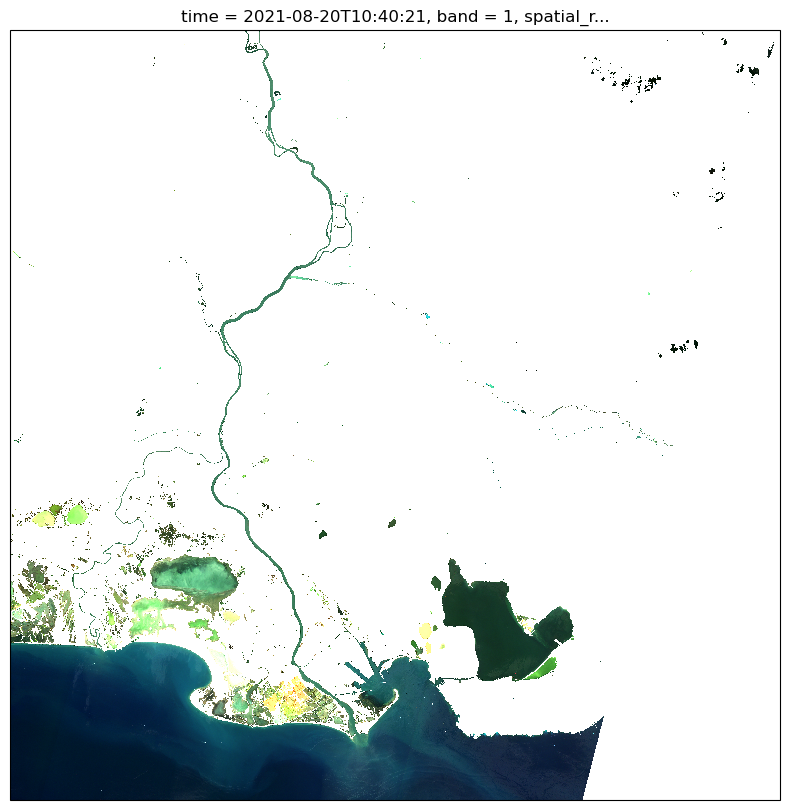
plt.figure(figsize=(10,10))
l2a.Rrs.sel(wl=[665,560,490]).where(l2a.mask==0).plot.imshow(rgb='wl', robust=True,subplot_kws=dict(projection=proj))
<matplotlib.image.AxesImage at 0x7f5ae31521f0>
/home/harmel/anaconda3/envs/grstbx/lib/python3.9/site-packages/matplotlib/cm.py:496: RuntimeWarning: invalid value encountered in cast
  xx = (xx * 255).astype(np.uint8)
Reprojection#
If you want to reproject in EPSG:4326 Geodetic coordinate system for World (not recommended)
l2a_reproj = l2a.rio.reproject(4326)
l2a_reproj
<xarray.Dataset>
Dimensions:             (x: 6477, y: 4695, wl: 11)
Coordinates:
  * x                   (x) float64 4.232 4.232 4.233 ... 5.626 5.626 5.626
  * y                   (y) float64 44.25 44.25 44.25 ... 43.24 43.24 43.24
    central_wavelength  (wl) float32 442.7 492.7 559.9 ... 1.614e+03 2.202e+03
  * wl                  (wl) int64 443 490 560 665 705 740 783 842 865 1610 2190
    time                datetime64[ns] 2021-08-20T10:40:21
    band                int64 1
    spatial_ref         int64 0
Data variables:
    Rrs                 (wl, y, x) float32 nan nan nan nan ... nan nan nan nan
    BRDFg               (y, x) float32 nan nan nan nan nan ... nan nan nan nan
    aot550              (y, x) float32 nan nan nan nan nan ... nan nan nan nan
    mask                (y, x) uint8 255 255 255 255 255 ... 255 255 255 255 255
    vza                 (y, x) float32 nan nan nan nan nan ... nan nan nan nan
    sza                 (y, x) float32 nan nan nan nan nan ... nan nan nan nan
    raa                 (y, x) float32 nan nan nan nan nan ... nan nan nan nan
    flags               (y, x) int64 0 0 0 0 0 0 0 0 0 0 ... 0 0 0 0 0 0 0 0 0 0
    dem                 (y, x) float32 nan nan nan nan nan ... nan nan nan nan
Attributes: (12/72)
    long_name:                           CA BLUE GREEN RED VRE_1 VRE_2 VRE_3 ...
    constellation:                       Sentinel-2
    constellation_id:                    S2
    product_path:                        /data/satellite/Sentinel-2/L1C/31TFJ...
    product_name:                        S2A_MSIL1C_20210820T104021_N0500_R00...
    product_filename:                    S2A_MSIL1C_20210820T104021_N0500_R00...
    ...                                  ...
    vis_swir_index_threshold:            0.0
    hcld_threshold:                      0.003
    dirdata:                             /data/grs/grsdata
    abs_gas_file:                        /home/harmel/Dropbox/Dropbox/work/gi...
    water_vapor_transmittance_file:      /home/harmel/Dropbox/Dropbox/work/gi...
metadata_profile: datacubeSubset with projected coordinates#
The easiest and fastest way to extract from lon/lat coordinates is to convert the lon/lat bounds into the projected coordinates in the geographic system of your image:
from pyproj import CRS, Transformer

lonmin,lonmax=4.92,5.3
latmin,latmax=43.6,43.35

in_crs = CRS.from_epsg(4326)
out_crs = CRS.from_epsg(l2a.rio.crs.to_epsg())

transform = Transformer.from_crs(in_crs, out_crs, always_xy=True)
minx,miny = transform.transform(lonmin, latmax)
maxx,maxy = transform.transform(lonmax, latmin)

l2a_subset = l2a.rio.clip_box(
    minx=minx,
    miny=miny,
    maxx=maxx,
    maxy=maxy)
l2a_subset
<xarray.Dataset>
Dimensions:             (wl: 11, x: 1502, y: 1428)
Coordinates:
  * wl                  (wl) int64 443 490 560 665 705 740 783 842 865 1610 2190
    time                datetime64[ns] 2021-08-20T10:40:21
  * x                   (x) float64 6.556e+05 6.556e+05 ... 6.856e+05 6.856e+05
  * y                   (y) float64 4.83e+06 4.83e+06 ... 4.801e+06 4.801e+06
    central_wavelength  (wl) float32 442.7 492.7 559.9 ... 1.614e+03 2.202e+03
    band                int64 1
    spatial_ref         int64 0
Data variables:
    Rrs                 (wl, y, x) float32 nan nan nan nan ... nan nan nan nan
    BRDFg               (y, x) float32 nan nan nan nan nan ... nan nan nan nan
    aot550              (y, x) float32 0.152 0.152 0.152 ... 0.172 0.172 0.172
    mask                (y, x) uint8 1 1 1 1 1 1 1 1 1 1 ... 1 1 1 1 1 1 1 1 1 1
    vza                 (y, x) float32 9.11 9.11 9.11 9.11 ... nan nan nan nan
    sza                 (y, x) float32 nan nan nan nan nan ... nan nan nan nan
    raa                 (y, x) float32 122.8 122.8 122.8 122.8 ... nan nan nan
    flags               (y, x) int64 512 512 512 512 512 ... 513 513 513 513 513
    dem                 (y, x) float32 46.0 46.0 45.0 45.0 ... 0.0 0.0 0.0 0.0
Attributes: (12/72)
    long_name:                           CA BLUE GREEN RED VRE_1 VRE_2 VRE_3 ...
    constellation:                       Sentinel-2
    constellation_id:                    S2
    product_path:                        /data/satellite/Sentinel-2/L1C/31TFJ...
    product_name:                        S2A_MSIL1C_20210820T104021_N0500_R00...
    product_filename:                    S2A_MSIL1C_20210820T104021_N0500_R00...
    ...                                  ...
    vis_swir_index_threshold:            0.0
    hcld_threshold:                      0.003
    dirdata:                             /data/grs/grsdata
    abs_gas_file:                        /home/harmel/Dropbox/Dropbox/work/gi...
    water_vapor_transmittance_file:      /home/harmel/Dropbox/Dropbox/work/gi...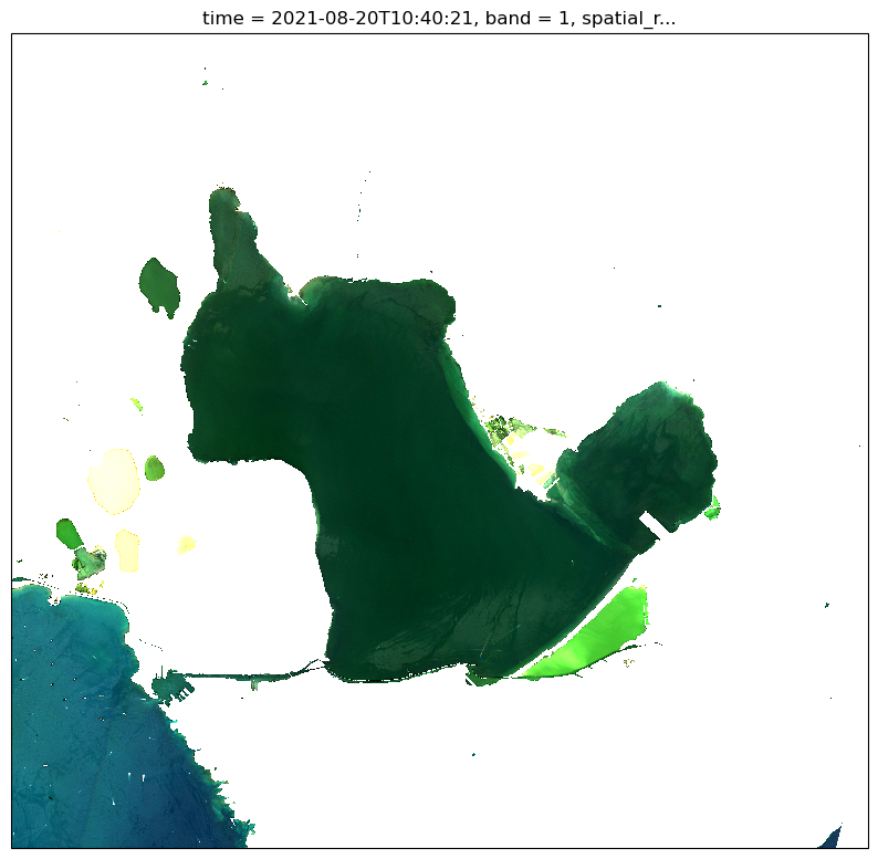
metadata_profile: datacubeplt.figure(figsize=(10,10))
l2a_subset.Rrs.sel(wl=[665,560,490]).where(l2a_subset.mask==0).plot.imshow(rgb='wl',
robust=True,
subplot_kws=dict(projection=proj))
<matplotlib.image.AxesImage at 0x7f5ae5eb80d0>
/home/harmel/anaconda3/envs/grstbx/lib/python3.9/site-packages/matplotlib/cm.py:496: RuntimeWarning: invalid value encountered in cast
  xx = (xx * 255).astype(np.uint8)
GRStbx#
Otherwise, I might be interested in using GRSTBX (Tristanovsk/grstbx) that provides the tools for subsettint and visualizing temporal datacubes
import grstbx
from grstbx import visual
import geopandas as gpd
import holoviews as hv
hv.extension('bokeh')


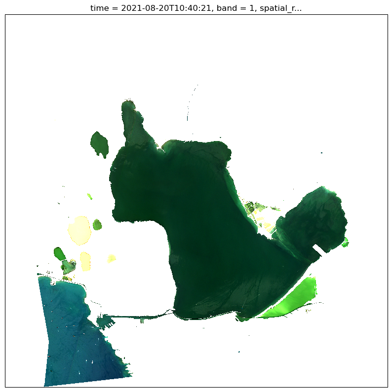
v=visual.ViewSpectral(l2a.Rrs,reproject=True)
The next cell will render the visualization tool. For subsetting, you can choose the polygon drawer tool on the right side and then press long to generate the polygon. Short clicks will add a new segment and long click end the polygon.
v.visu()
The next cell was commented for rendendering in Readthedocs (please uncomment for proper use of the notebook)
#geom_ = v.get_geom(v.aoi_stream,crs=l2a.rio.crs)
#geom_.to_file("roi_grs_visu_simple.json", driver="GeoJSON")
geom_ = gpd.read_file("roi_grs_visu_simple.json", driver="GeoJSON")
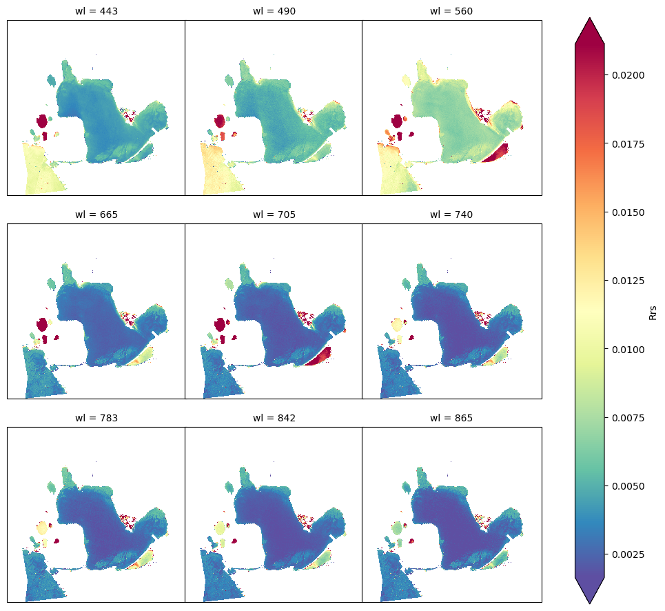
Rrs_clipped = l2a.Rrs.sel(wl=slice(400,1000)).where(l2a.mask==0).rio.clip(geom_.geometry.values)
plt.figure(figsize=(10,10))
Rrs_clipped.sel(wl=[665,560,490]).plot.imshow(rgb='wl',
                                              robust=True,
                                              subplot_kws=dict(projection=proj))
<matplotlib.image.AxesImage at 0x7f5c0a526070>
/home/harmel/anaconda3/envs/grstbx/lib/python3.9/site-packages/matplotlib/cm.py:496: RuntimeWarning: invalid value encountered in cast
  xx = (xx * 255).astype(np.uint8)
Rrs_clipped.plot.imshow(col='wl',col_wrap=3, robust=True, cmap=plt.cm.Spectral_r,
                                              subplot_kws=dict(projection=proj))
<xarray.plot.facetgrid.FacetGrid at 0x7f5c23ac33d0>