Simple use of GRS API

Contents

Simple use of GRS API#

import os

import matplotlib as mpl
import matplotlib.pyplot as plt

import numpy as np
import xarray as xr

import cartopy.crs as ccrs

# import the GRS package suite
import GRSdriver
import grs 
#import grstbx

print(f'-GRSdriver: {GRSdriver.__version__}')
print(f'-grs: {grs.__version__}')
#print(f'-grstbx: {grstbx.__version__}')

-GRSdriver: 1.0.3
-grs: 2.1.6

Set the path of your Sentinel-2 image and corresponding CAMS and DEM files#

file = '/data/satellite/Sentinel-2/L1C/30PYT/2018/10/19/S2A_MSIL1C_20181019T102031_N0500_R065_T30PYT_20230815T043850.SAFE'

tile = file.split('_')[-2][1:]
dem_file = '/home/harmel/Dropbox/Dropbox/satellite/dem/COP-DEM_GLO-30-DGED_'+tile+'.tif'
cams_file = '/data/cams/world/cams_forecast_2018-10.nc'

Apply next cell if you want to save the output L2A image into the GRS format.#

process_.ofile='/data/satellite/grs_v21_test_image'
process_.write_output()

INFO:root:export final product into netcdf
INFO:root:export into encoded netcdf

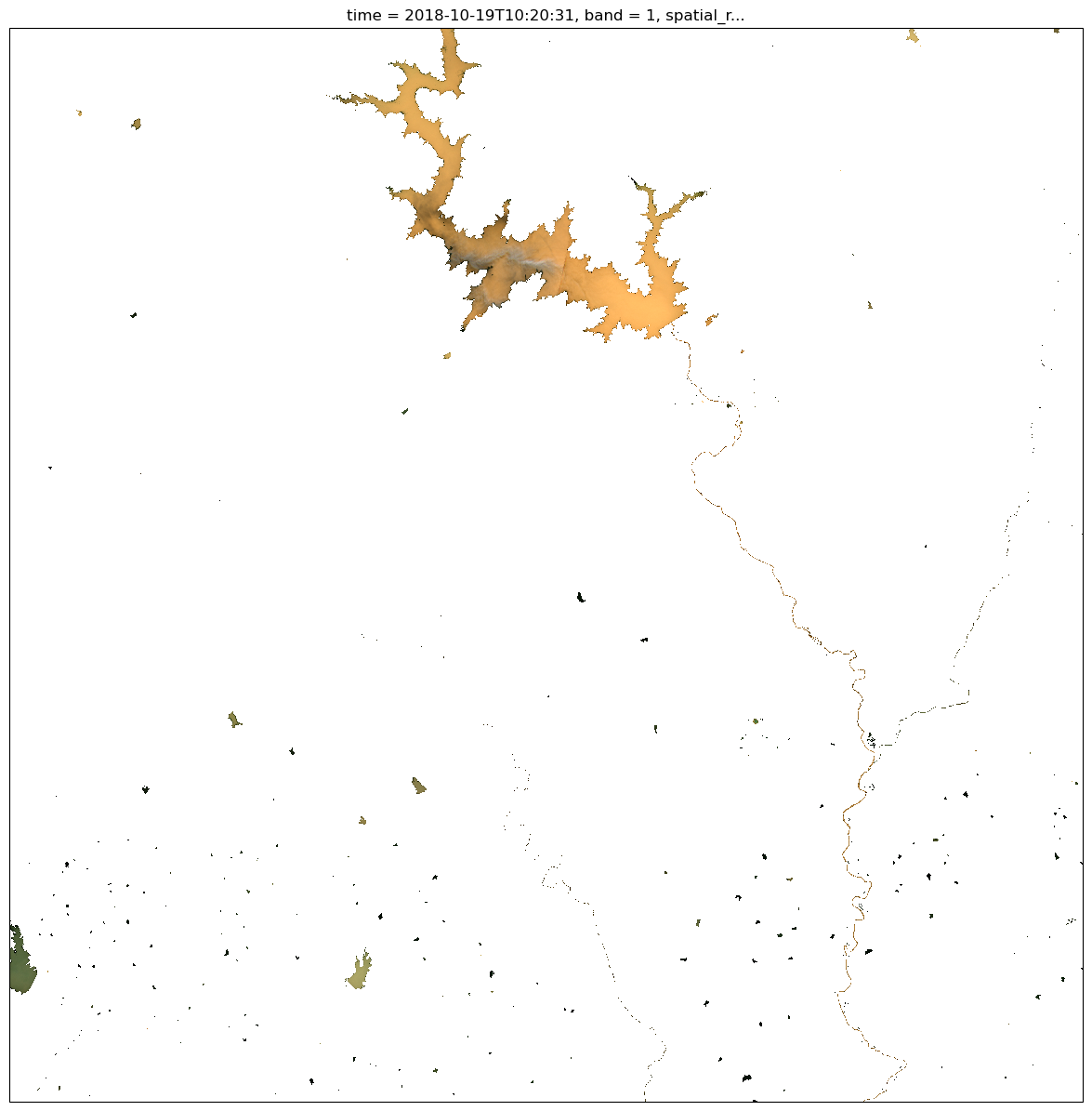
You can then easily plot the corrected images from the remote sensing reflectance, \(R_{rs}\ (sr^{-1})\).#

str_epsg = str(process_.l2a.l2_prod.rio.crs)
zone = str_epsg[-2:]
is_south = str_epsg[2] == 7
proj = ccrs.UTM(zone, is_south)

plt.figure(figsize=(15,15))
process_.l2a.l2_prod.Rrs.sel(wl=[665,560,490]).plot.imshow(rgb='wl', robust=True,subplot_kws=dict(projection=proj))

<matplotlib.image.AxesImage at 0x7fba970c2a00>

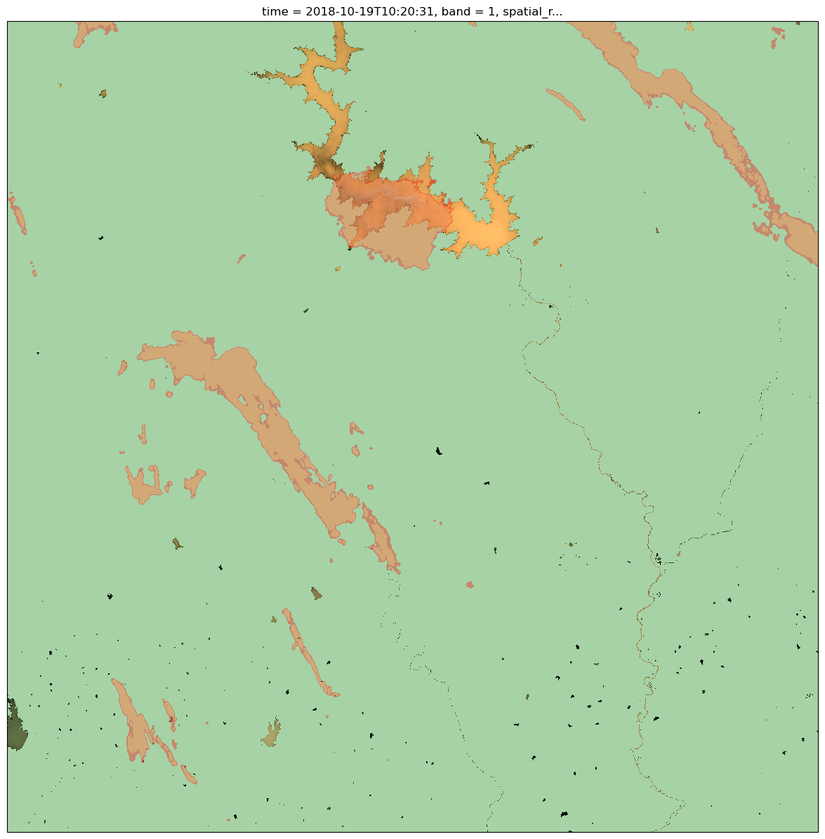
../_images/e4c6b65139731d901931757c86601bf02d151182e073c37e6671607ee2f00116.png

Then, you can check the flags#

raster = process_.l2a.l2_prod
str_epsg = str(process_.l2a.l2_prod.rio.crs)
zone = str_epsg[-2:]
is_south = str_epsg[2] == 7
proj = ccrs.UTM(zone, is_south)


alpha=0.35
bcmap = mpl.colors.ListedColormap([(0,0,0,0),'khaki'])
bcmap2 = mpl.colors.ListedColormap([(0,0,0,0),'red'])

plt.figure(figsize=(15,15))
raster.Rrs.sel(wl=[665,560,490]).plot.imshow(rgb='wl', robust=True,subplot_kws=dict(projection=proj))

# get landmask (third bit)
bcmap = mpl.colors.ListedColormap([(0,0,0,0),'green'])
flag_value = 1 << 3
((raster.flags_l1c & flag_value) != 0).plot.imshow(cmap=bcmap,alpha=alpha,add_colorbar=False)
# get cloud p06 (second bit)
bcmap = mpl.colors.ListedColormap([(0,0,0,0),'red'])
flag_value = int('0010', 2)
((raster.flags_l1c & flag_value) != 0).plot.imshow(cmap=bcmap,alpha=alpha,add_colorbar=False)
# get cloud p08 (third bit)
bcmap = mpl.colors.ListedColormap([(0,0,0,0),'khaki'])
flag_value = int('0100', 2)
((raster.flags_l1c & flag_value) != 0).plot.imshow(cmap=bcmap,alpha=alpha,add_colorbar=False)

<matplotlib.image.AxesImage at 0x7fba97122c10>

../_images/ce30996969fe39feb887bcfbabb535a173bff4a9a0fffc017c89f0230c690b11.png

You can also check the shade from the elevation from the digital elevation model (DEM)#

azi = raster.attrs[‘mean_solar_azimuth’] sza = raster.attrs[‘mean_solar_zenith_angle’] dem_attrs = grstbx.dem.compute_dem_attributes(raster.dem,sza,azi)

plt.figure(figsize=(15,15)) dem_attrs.shaded.plot.imshow(robust=True,subplot_kws=dict(projection=proj),cmap=plt.cm.Greys_r,cbar_kwargs={‘shrink’:0.4}) process_.l2a.l2_prod.Rrs.sel(wl=[665,560,490]).plot.imshow(rgb=‘wl’, robust=True,subplot_kws=dict(projection=proj))

Finally you can mask your image from the desired combination of flags#

# get cloud p08 (third bit)

flag_value = 1 << 2
mask = ((raster.flags_l1c & flag_value) != 0)
Rrs = process_.l2a.l2_prod.Rrs.where(~mask)

plt.figure(figsize=(15,15))
#dem_attrs.shaded.plot.imshow(robust=True,subplot_kws=dict(projection=proj),cmap=plt.cm.Greys_r,cbar_kwargs={'shrink':0.4})
Rrs.sel(wl=[665,560,490]).plot.imshow(rgb='wl', robust=True,subplot_kws=dict(projection=proj))

<matplotlib.image.AxesImage at 0x7fba96907430>

../_images/ce343cca19bca0fcff3dd97192bee25d47464e0b288d5e43b27073616d28ff4d.png