Development example for GRS step-by-step application to Landsat images#
'''
Main program
'''

import os
import glob

import matplotlib as mpl
import matplotlib.pyplot as plt

import numpy as np
import xarray as xr
import pandas as pd

import logging

import panel as pn

import cartopy.crs as ccrs
import geopandas as gpd

import GRSdriver
import grs
from grs import Product, AuxData, acutils, CamsProduct, L2aProduct, Rasterization
import grstbx
from grstbx import visual

pn.extension()
opj = os.path.join

print(f'-GRSdriver: {GRSdriver.__version__}')
print(f'-grs: {grs.__version__}')
print(f'-grstbx: {grstbx.__version__}')


-GRSdriver: 1.0.4
-grs: 2.1.6
-grstbx: 2.0.2
Indicate the path where you put the look-up table file#
lut_file = '/data/vrtc/xlut/toa_lut_opac_wind_light.nc'
lut_file = '/data/vrtc/xlut/toa_lut_opac_wind_light_v2.nc'
trans_lut_file = '/data/vrtc/xlut/transmittance_lut_opac_wind_light_v2.nc'
Set the path of your Sentinel-2 image and corresponding CAMS file#
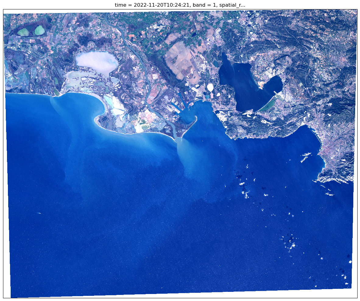
file ='/data/satellite/landsat/LC09_L1TP_196030_20221120_20230321_02_T1'

file_nc = file+'.nc'

cams_file = '/data/cams/world/cams_forecast_2022-11.nc'
l1c = GRSdriver.LandsatDriver(file)
l1c.INFO
| bandId | 0 | 1 | 2 | 3 | 4 | 5 | 6 | 7 | 8 |
|---|---|---|---|---|---|---|---|---|---|
| ESA | B01 | B02 | B03 | B08 | B04 | B05 | B09 | B06 | B07 |
| EOREADER | CA | BLUE | GREEN | PAN | RED | NIR | SWIR_CIRRUS | SWIR_1 | SWIR_2 |
| Wavelength (nm) | 443 | 490 | 560 | 590 | 665 | 865 | 1370 | 1610 | 2190 |
| Band width (nm) | 25 | 60 | 60 | 173 | 33 | 28 | 21 | 95 | 287 |
| Resolution (m) | 30 | 30 | 30 | 15 | 30 | 30 | 30 | 30 | 30 |
l1c.load_mask()
l1c.load_product()
/home/harmel/anaconda3/envs/grstbx/lib/python3.9/site-packages/xarray/core/indexes.py:659: RuntimeWarning: '<' not supported between instances of 'SpectralBandNames' and 'SpectralBandNames', sort order is undefined for incomparable objects.
  new_pd_index = pd_indexes[0].append(pd_indexes[1:])
prod = Product(l1c.prod)
prod.raster
<xarray.Dataset>
Dimensions:      (x: 7671, y: 7791, wl: 9, wl_hr: 2951)
Coordinates:
  * x            (x) float64 5.349e+05 5.349e+05 5.35e+05 ... 7.65e+05 7.65e+05
  * y            (y) float64 4.899e+06 4.899e+06 ... 4.666e+06 4.666e+06
    spatial_ref  int64 0
  * wl           (wl) int64 443 490 560 590 665 865 1370 1610 2190
  * wl_hr        (wl_hr) float64 400.0 401.0 402.0 ... 1.35e+04 1.35e+04
    time         datetime64[ns] 2022-11-20T10:24:21
    band         int64 1
Data variables:
    bands        (wl, y, x) float32 nan nan nan nan nan ... nan nan nan nan nan
    SRF          (wl, wl_hr) float64 ...
    wl_true      (wl) float64 442.8 482.3 560.9 ... 1.608e+03 2.201e+03
    sza          (y, x) float32 nan nan nan nan nan nan ... nan nan nan nan nan
    vza          (y, x) float32 nan nan nan nan nan nan ... nan nan nan nan nan
    raa          (y, x) float32 nan nan nan nan nan nan ... nan nan nan nan nan
    l1c_flag     (y, x) uint32 1 1 1 1 1 1 1 1 1 1 1 1 ... 1 1 1 1 1 1 1 1 1 1 1
    surfwater    (y, x) int8 1 1 1 1 1 1 1 1 1 1 1 1 ... 1 1 1 1 1 1 1 1 1 1 1 1
Attributes: (12/20)
    long_name:              CA BLUE GREEN PAN RED NIR SWIR_CIRRUS SWIR_1 SWIR_2
    constellation:          Landsat-9
    constellation_id:       L9
    product_path:           /data/satellite/landsat/LC09_L1TP_196030_20221120...
    product_name:           LC09_L1TP_196030_20221120_20230321_02_T1
    product_filename:       LC09_L1TP_196030_20221120_20230321_02_T1
    ...                     ...
    satellite:              Landsat-9
    solar_irradiance:       NA
    solar_irradiance_unit:  W/m²/µm
    processing_time:        2024-04-19T09:57:08.676420
    processor:              grs_2.1.6
version: 2.1.6Load the image and convert it into netcdf for further fatest loading (not necessary)#
#l1c.prod.to_netcdf(file_nc)
#prod = Product(xr.open_dataset(file_nc))
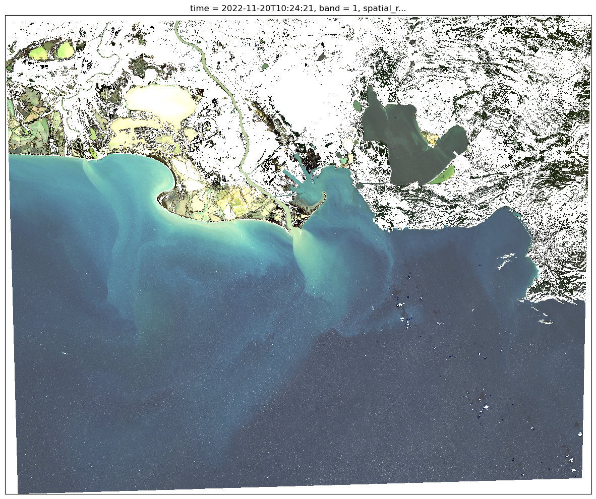
Visualize, interact and subset your region of interest#
Yuo can use the “polygon” tool to subset the image and proceed with further processing
v=visual.view_spectral(prod.raster.bands,reproject=True)
v.title="## Landsat-9 L1C"
v.minmaxvalues=(0,0.3)
v.minmax=[0,0.5]
v.visu()
You can save the area of interest into a json file for reuse (uncomment the next two cells)
#geom_ = v.get_geom(v.aoi_stream,crs=prod.raster.rio.crs)
#geom_.to_file("roi_example.json", driver="GeoJSON")
geom_ = gpd.read_file("roi_example.json", driver="GeoJSON")
raster_clipped = xr.Dataset()
prod.raster.bands.rio.clip(geom_.geometry.values)
for param in prod.raster.keys():
    da = prod.raster[param]
    if 'x' in da.dims and 'y' in da.dims:
        raster_clipped[param]=da.rio.clip(geom_.geometry.values)
    else:
        raster_clipped[param]=da
raster_clipped.attrs = prod.raster.attrs
str_epsg = str(raster_clipped.rio.crs)
zone = str_epsg[-2:]
is_south = str_epsg[2] == 7
proj = ccrs.UTM(zone, is_south)

plt.figure(figsize=(15,15))
raster_clipped.bands.sel(wl=[665,560,490]).plot.imshow(rgb='wl', robust=True,subplot_kws=dict(projection=proj))
<matplotlib.image.AxesImage at 0x7fd7bbd2e550>
Start GRS processing#
If you want to process the whole tile comment the following line
prod.raster = raster_clipped
Set sensor specific parameters
if 'S2' in prod.sensor:
    monoview = False
else:
    monoview = True
_R_ = Rasterization(monoview=monoview)
Start by checking the CAMS data
##################################
# GET ANCILLARY DATA (Pressure, O3, water vapor, NO2...
##################################
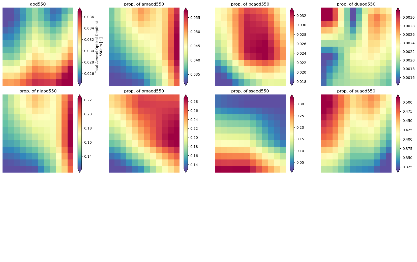
cams = CamsProduct(prod.raster, cams_file=cams_file)
#cams.wls=[355,380,400,440,469,500, 550, 645,670,800, 865,1020, 1240,1640,2130]
cams.load()
params=['aod550','amaod550', 'bcaod550', 'duaod550', 'niaod550', 'omaod550', 'ssaod550', 'suaod550']
Nrows = (len(params) + 4) // 4
fig, axs = plt.subplots(Nrows, 4, figsize=(4 * 4.2, Nrows * 3.5))
axs = axs.ravel()
[axi.set_axis_off() for axi in axs]
aod550 = cams.raster['aod550']
aod550
for i, param in enumerate(params):
    if i == 0:
        fig = cams.raster[param].plot.imshow(robust=True, ax=axs[i],cmap=plt.cm.Spectral_r)
        fig.axes.set_title(param)
    else:
        fig = (cams.raster[param]/aod550).plot.imshow(robust=True, ax=axs[i],cmap=plt.cm.Spectral_r)
        fig.axes.set_title('prop. of '+param)
    #fig.colorbar.set_label(self.raster[param].units)
    fig.axes.set(xticks=[], yticks=[])
    fig.axes.set_ylabel('')
    fig.axes.set_xlabel('')
plt.tight_layout()
#cams.plot_params(params=['aod550', 'aod2130', 'ssa550', 't2m', 'msl', 'sp','tcco', 'tchcho', 'tc_oh', 'tc_ch4', 'tcno2', 'gtco3', 'tc_c3h8', 'tcwv', 'u10', 'v10'], cmap=plt.cm.Spectral_r)
#'ammonium_aerosol_optical_depth_550nm', 'black_carbon_aerosol_optical_depth_550nm',
#                'dust_aerosol_optical_depth_550nm',
#                'nitrate_aerosol_optical_depth_550nm', 'organic_matter_aerosol_optical_depth_550nm',
#                'sea_salt_aerosol_optical_depth_550nm',
#                'sulphate_aerosol_optical_depth_550nm',
cams.plot_params(params=['v10','u10', 'msl', 'sp','t2m', 'tcco', 'tc_ch4', 'tcno2', 'gtco3', 'tcwv',
 'amaod550', 'bcaod550', 'duaod550', 'niaod550', 'omaod550', 'ssaod550', 'suaod550',
 'aod1240', 'aod469', 'aod550', 'aod670', 'aod865',

 ],


                 cmap=plt.cm.Spectral_r)
plt.show()

cams.raster
<xarray.Dataset>
Dimensions:      (y: 12, x: 12)
Coordinates:
    time         datetime64[ns] 2022-11-20T10:24:21
    band         int64 1
  * x            (x) float64 5.989e+05 6.083e+05 ... 6.926e+05 7.02e+05
  * y            (y) float64 4.837e+06 4.829e+06 ... 4.761e+06 4.753e+06
    spatial_ref  int64 0
Data variables: (12/22)
    v10          (y, x) float64 -4.492 -4.857 -5.251 ... -10.16 -9.777 -9.391
    t2m          (y, x) float64 283.8 284.0 284.0 283.9 ... 285.3 285.3 285.3
    msl          (y, x) float64 1.016e+05 1.016e+05 ... 1.014e+05 1.014e+05
    sp           (y, x) float64 1.005e+05 1.008e+05 ... 1.01e+05 1.009e+05
    amaod550     (y, x) float64 0.0009109 0.0009924 ... 0.00184 0.002093
    bcaod550     (y, x) float64 0.000607 0.0006342 ... 0.0009194 0.0009528
    ...           ...
    tcco         (y, x) float64 0.0007466 0.0007487 ... 0.000738 0.0007368
    tc_ch4       (y, x) float64 0.0103 0.01033 0.01035 ... 0.01036 0.01035
    tcno2        (y, x) float64 1.821e-06 1.902e-06 ... 2.602e-06 2.694e-06
    gtco3        (y, x) float64 0.006238 0.006244 0.006251 ... 0.006332 0.006348
    tcwv         (y, x) float64 7.95 7.996 8.037 8.068 ... 7.718 7.749 7.781
    u10          (y, x) float64 2.583 2.488 2.442 2.467 ... 6.908 7.015 7.121
Attributes:
    Conventions:  CF-1.6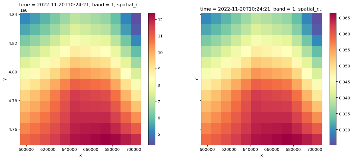
history: 2024-02-21 18:34:02 GMT by grib_to_netcdf-2.25.1: /opt/ecmw...You may also want to visualize the module wind speed or the mean square slope (sigma2 taken from the Cox Munk isotropic model)
wind = np.sqrt(cams.raster['v10']**2+cams.raster['u10']**2)
sigma2=(wind+0.586)/195.3

fig,axs = plt.subplots(1,2,figsize=(15,6),sharey=True,sharex=True)
wind.plot.imshow(ax=axs[0],cmap=plt.cm.Spectral_r)
sigma2.plot.imshow(ax=axs[1],cmap=plt.cm.Spectral_r)
<matplotlib.image.AxesImage at 0x7fd7b91f5f40>
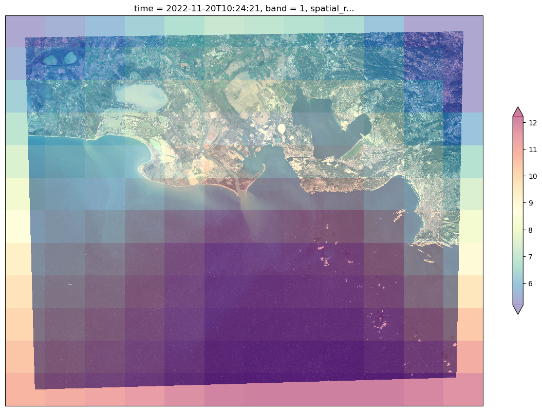
You can also plot a cams parameter as a new layer above the S2 RGB image
plt.figure(figsize=(15,15))

prod.raster.bands.sel(wl=[665,560,490]).plot.imshow(rgb='wl', robust=True,subplot_kws=dict(projection=proj))
wind.plot.imshow( cmap=plt.cm.Spectral_r,robust=True,alpha=0.5,subplot_kws=dict(projection=proj),cbar_kwargs={'shrink':0.35})
<matplotlib.image.AxesImage at 0x7fd7b8c9a490>
Take the mean values for LUT selection and interpolation
_sigma2 = sigma2.mean().values
_wind = wind.mean().values
print(_sigma2,_wind)
0.050103689208529464 9.199250502425805
Prepare spectral bands for further processing and load LUT Set parameter ‘wl_to_process’
#####################################
# SUBSET RASTER TO KEEP REQUESTED BANDS
#####################################
if prod.bcirrus:
    prod.cirrus = prod.raster.bands.sel(wl=prod.bcirrus, method='nearest')
if prod.bwv:
    prod.wv = prod.raster.bands.sel(wl=prod.bwv, method='nearest')
prod.raster = prod.raster.sel(wl=prod.wl_process, method='nearest')
#####################################
# LOAD LUT FOR ATMOSPHERIC CORRECTION
#####################################
#logging.info('loading lut...' + prod.lutfine)

Ttot_Ed = xr.open_dataset(trans_lut_file)
Ttot_Ed['wl'] = Ttot_Ed['wl'] * 1000

aero_lut = xr.open_dataset(lut_file)
aero_lut['wl']=aero_lut['wl']*1000
aero_lut['aot'] = aero_lut.aot.isel(wind=0).squeeze()
# remove URBAN aerosol model for this example.drop_sel(model='URBA_rh70')
models=aero_lut.drop_sel(model='URBA_rh70').model.values
#aero_lut
wl_true = prod.raster.wl_true
_auxdata = AuxData(wl=wl_true)#wl=masked.wl)
sunglint_eps = _auxdata.sunglint_eps#['mean'].interp(wl=wl_true)
rot = _auxdata.rot#.interp(wl=wl_true)
Set aerosol model from CAMS data#
Get spectral aerosol optical thickness from CAMS raster
cams_aot_mean = cams.cams_aod.mean(['x','y'])
cams_aot_ref = cams.cams_aod.interp(wl=550,method='quadratic').compute()
cams_aot_ref_mean =  cams_aot_ref.mean(['x','y'])
Check proximity with tabulated models (LUT) and select representative aerosol model
fig, axs = plt.subplots(1, 2, figsize=(18, 4.5))
aero_lut.aot.sel(model=models,aot_ref=1).plot(ax=axs[0],hue='model')#,add_legend=False)
(cams_aot_mean/cams_aot_ref_mean).plot(ax=axs[0],color='black')
aero_lut.aot.isel(model=[4,2]).mean('model').sel(aot_ref=1).plot(ax=axs[0],color='grey')
lut_aod=aero_lut.aot.sel(model=models,aot_ref=1).interp(wl=cams.cams_aod.wl)
rank = np.abs((cams_aot_mean/cams_aot_ref_mean)-lut_aod).sum('wl')
axs[1].bar(x=rank.model, height=rank.values)
plt.xticks(rotation=30, ha='right')
plt.show()

idx = np.abs((cams_aot_mean/cams_aot_ref_mean)-lut_aod).sum('wl').argmin()
opac_model = aero_lut.sel(model=models).model.values[idx]
print(opac_model)
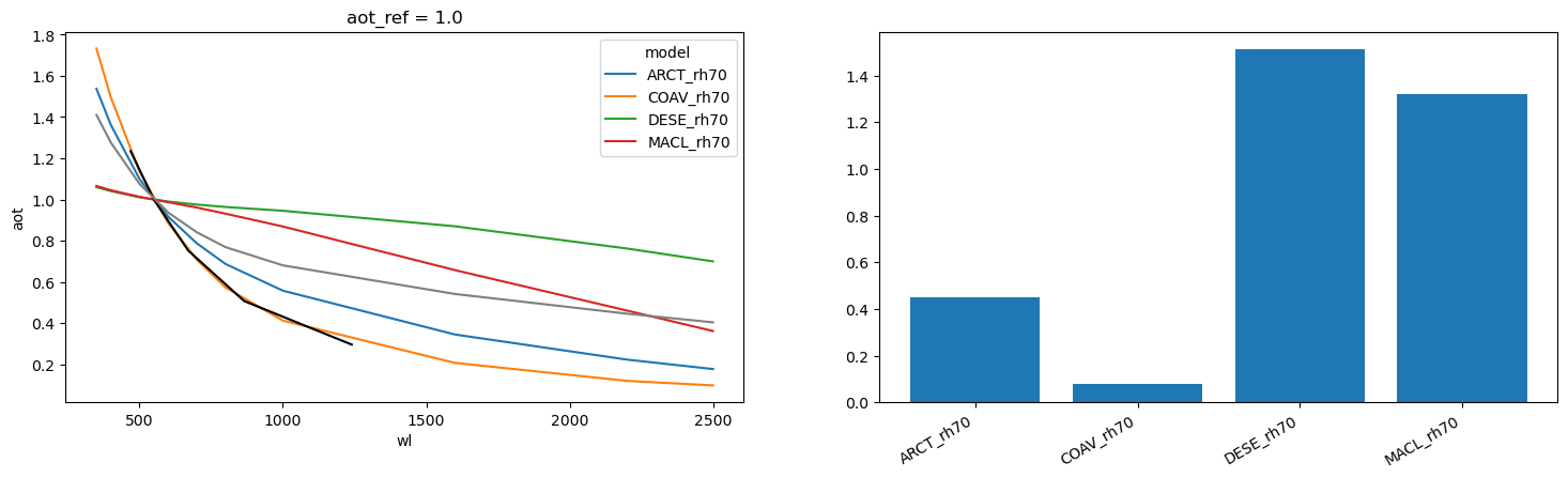
COAV_rh70
absorbing gases correction#
gas_trans = acutils.GaseousTransmittance(prod, cams)
Tg_raster = gas_trans.get_gaseous_transmittance()
#Tg_raster
logging.info('correct for gaseous absorption')
for wl in prod.raster.wl.values:
    Tg_ = Tg_raster.sel(wl=wl).interp(x=prod.raster.x, y=prod.raster.y)
    prod.raster['bands'].loc[wl] = prod.raster.bands.sel(wl=wl) / Tg_
    del Tg_
prod.raster.bands.attrs['gas_absorption_correction'] = True
INFO:root:correct for gaseous absorption
import gc
gc.collect()
158195
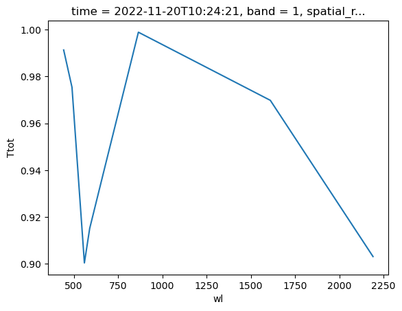
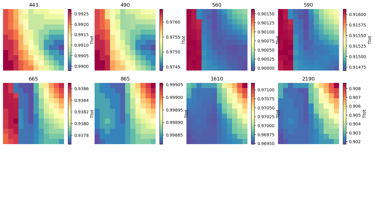
You can check the gaseous transmittance for each spectral band
plt.figure()
Tg_raster.mean('x').mean('y').plot()
fig,axs = plt.subplots(3,4,figsize=(15,9),sharey=True,sharex=True)
axs=axs.ravel()
[axi.set_axis_off() for axi in axs]
for iwl in range(len(prod.wl_process)):
    #axs[iwl].set_axis_on()
    Tg_raster.isel(wl=iwl).plot(ax=axs[iwl],cmap=plt.cm.Spectral_r)
    axs[iwl].set_title( str(Tg_raster.isel(wl=iwl).wl.values))
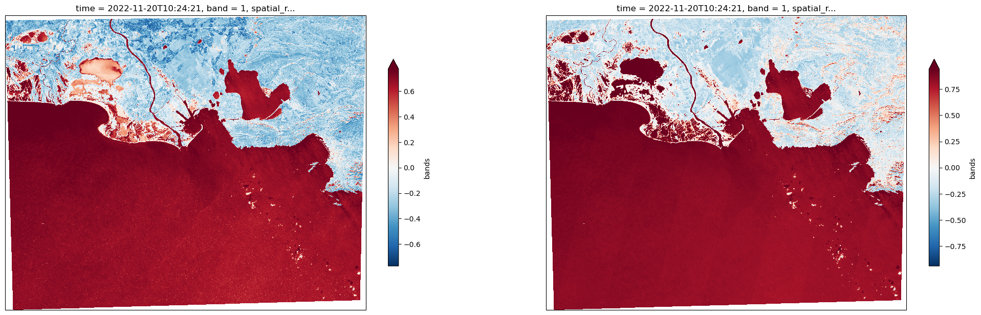
Water mask#
# Compute NDWI

#green = prod.raster.bands.sel(wl=565,method='nearest')
#nir = prod.raster.bands.sel(wl=prod.b865)

green = prod.raster.bands.sel(wl=prod.bvis,method='nearest')
nir = prod.raster.bands.sel(wl=prod.bnir,method='nearest')#prod.b865)
swir = prod.raster.bands.sel(wl=prod.bswir)
b2200 = prod.raster.bands.sel(wl=prod.bswir2)

ndwi = (green - nir) / (green + nir)
ndwi_swir = (green - swir) / (green + swir)

prod.raster['ndwi'] = ndwi
prod.raster.ndwi.attrs = {
'description': 'Normalized difference spectral index between bands at ' + str(prod.bvis) + ' and ' + str(
    prod.bnir) + ' nm', 'units': '-'}
prod.raster['ndwi_swir'] = ndwi_swir
prod.raster.ndwi_swir.attrs = {
'description': 'Normalized difference spectral index between bands at ' + str(prod.bvis) + ' and ' + str(
    prod.bswir) + ' nm', 'units': '-'}
fig = plt.figure(figsize=(25, 15))
ax = plt.subplot(1, 2, 1, projection=proj)
ndwi.plot.imshow(robust=True,subplot_kws=dict(projection=proj),cbar_kwargs={'shrink':0.35})#,vmin=-0.1,vmax=0.1,cmap=plt.cm.RdBu_r)
ax = plt.subplot(1, 2, 2, projection=proj)
ndwi_swir.plot.imshow(robust=True,subplot_kws=dict(projection=proj),cbar_kwargs={'shrink':0.35})#,vmin=-0.1,vmax=0.1,cmap=plt.cm.RdBu_r)
<matplotlib.image.AxesImage at 0x7fd7b956ffa0>
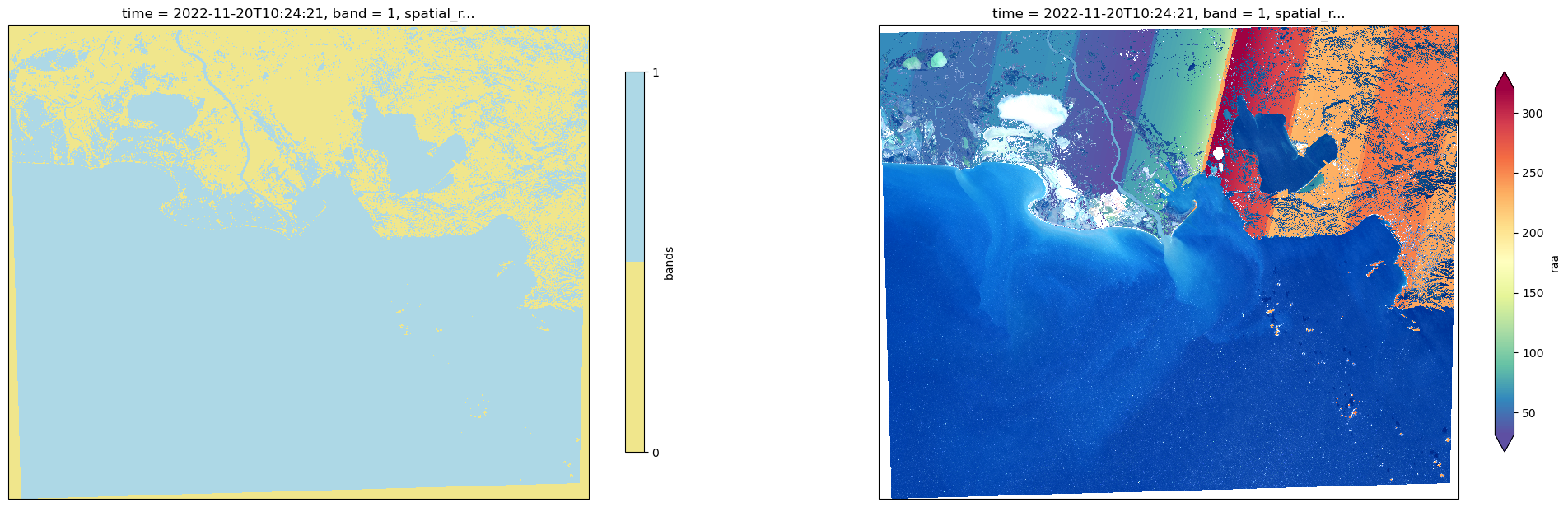
mask =  (ndwi_swir > 0) &  (b2200 < 0.2)#(ndwi > -0.0) &
masked = prod.raster.bands.where(mask)

from matplotlib.colors import ListedColormap
# binary cmap
bcmap = ListedColormap(['khaki', 'lightblue'])
xmask = xr.where(mask,1,0)

fig = plt.figure(figsize=(25, 15))
ax = plt.subplot(1, 2, 1, projection=proj)
xmask.plot.imshow(ax=ax,cmap=bcmap, cbar_kwargs={'ticks': [0, 1], 'shrink': 0.4})
ax = plt.subplot(1, 2, 2, projection=proj)
prod.raster['raa'].plot.imshow(cmap=plt.cm.Spectral_r, ax=ax, robust=True,cbar_kwargs={'shrink':0.4})
masked.sel(wl=[665,560,490]).plot.imshow(rgb='wl', robust=True,ax=ax)
<matplotlib.image.AxesImage at 0x7fd7bb448d60>
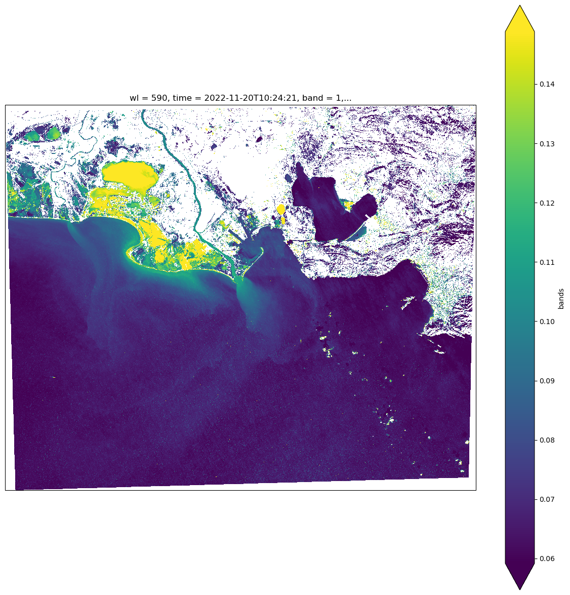
plt.figure(figsize=(15,15))

masked.sel(wl=590).plot.imshow( robust=True,subplot_kws=dict(projection=proj))
<matplotlib.image.AxesImage at 0x7fd7b95fb3a0>
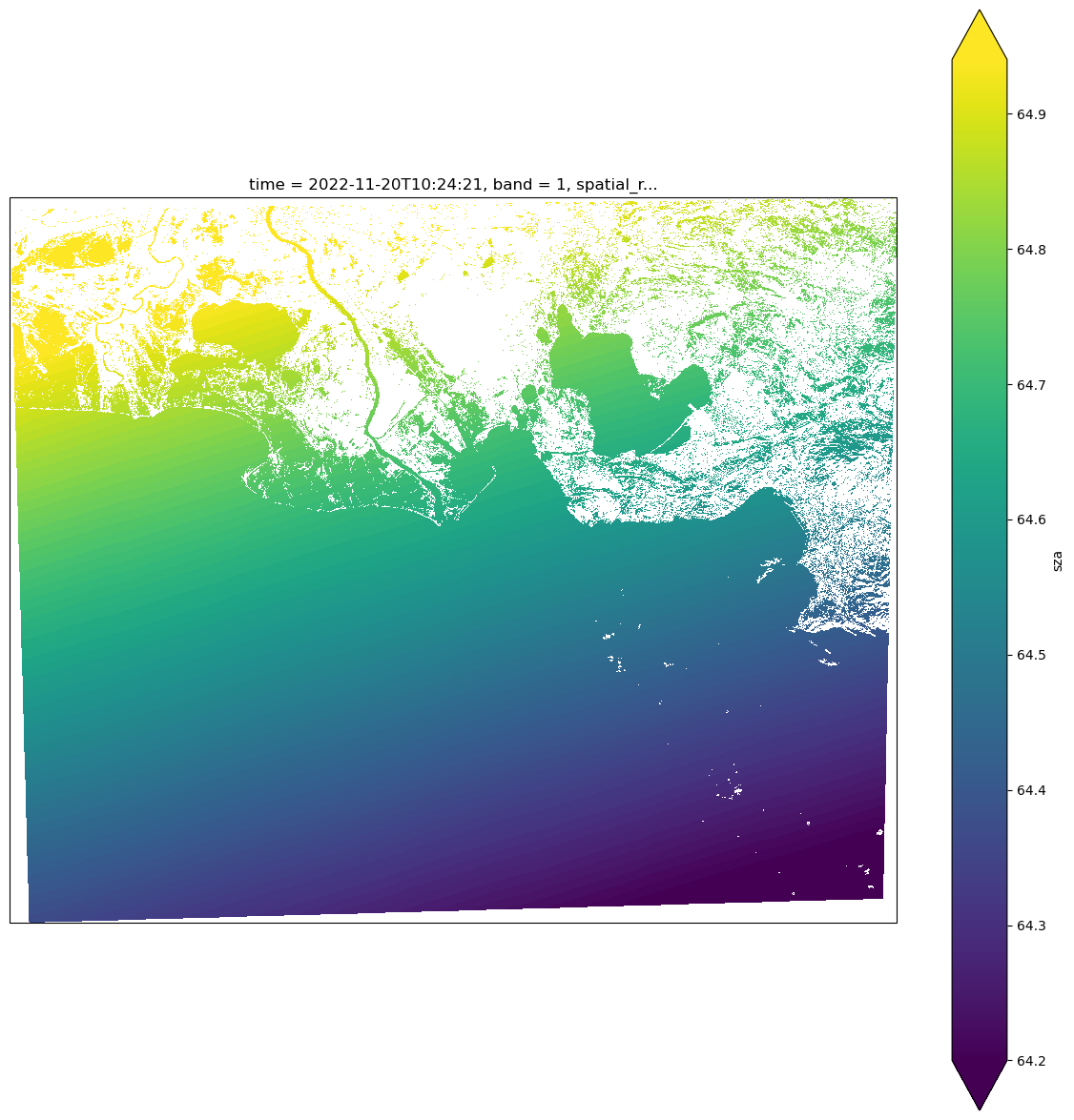
If you are happy with your mask you continue and proceed with masking, tweak the threshold values again, otherwise.
prod.raster['bands'] = masked
prod.raster['sza'] =  prod.raster['sza'].where(mask)


plt.figure(figsize=(15,15))
prod.raster['sza'].plot.imshow( robust=True,subplot_kws=dict(projection=proj))
<matplotlib.image.AxesImage at 0x7fd7bb079fd0>
Preparation of LUT and other input parameters
aero_lut.model
<xarray.DataArray 'model' (model: 5)>
array(['ARCT_rh70', 'COAV_rh70', 'DESE_rh70', 'MACL_rh70', 'URBA_rh70'],
      dtype=object)
Coordinates:
* model (model) object 'ARCT_rh70' 'COAV_rh70' ... 'MACL_rh70' 'URBA_rh70'models = ['ARCT_rh70', 'COAV_rh70', 'DESE_rh70', 'MACL_rh70', 'URBA_rh70']
Nwl,height,width = prod.raster.bands.shape
chunk = 256
pressure_ref=101500.
cams_aot_ref = cams.cams_aod.interp(wl=550,method='quadratic').compute() #*0.7#.interp(x=prod.raster.x,y=prod.raster.y).compute()#.plot.imshow()
aot_ref_raster = cams_aot_ref
iwl_swir = [-2, -1]
aero_lut_=aero_lut.sel(wind=_wind,method='nearest').sel(model=opac_model)#.isel(model=[4,2]).mean('model') # #opac_model)
aero_lut_
<xarray.Dataset>
Dimensions:            (aot_ref: 10, wl: 10, sza: 45, vza: 14, azi: 73)
Coordinates:
  * wl                 (wl) float32 350.0 400.0 500.0 ... 2.2e+03 2.5e+03
  * aot_ref            (aot_ref) float32 0.0 0.001 0.01 0.1 ... 0.5 0.7 1.0 1.5
  * sza                (sza) float32 0.0 2.0 4.0 6.0 8.0 ... 82.0 84.0 86.0 88.0
    wind               float64 8.0
  * vza                (vza) float32 0.0 1.14 2.62 4.11 ... 16.06 17.55 19.05
  * azi                (azi) float32 0.0 5.0 10.0 15.0 ... 350.0 355.0 360.0
    model              <U9 'COAV_rh70'
Data variables: (12/18)
    wl_ref             (aot_ref, wl) float32 ...
    Cext_ref           (aot_ref, wl) float32 ...
    ssa_ref            (aot_ref, wl) float32 ...
    aot                (aot_ref, wl) float32 ...
    Cext               (aot_ref, wl) float32 ...
    ssa                (aot_ref, wl) float32 ...
    ...                 ...
    Eu                 (aot_ref, wl, sza) float32 ...
    Eo                 (aot_ref, wl, sza) float32 ...
    Eddir              (aot_ref, wl, sza) float32 ...
    Eudir              (aot_ref, wl, sza) float32 ...
    Eodir              (aot_ref, wl, sza) float32 ...
I (aot_ref, wl, sza, vza, azi) float32 ...ang_resol={'sza':0.1, 'vza':0.1, 'raa_round':0}
szamin,szamax=float(prod.raster['sza'].min()),float(prod.raster['sza'].max())
vzamin,vzamax=float(prod.raster.isel(wl=0)['vza'].min()),float(prod.raster.isel(wl=0)['vza'].max())
# check for out-of-range
def check_out_of_range(vmin,vmax,ceiling=88):
vmin = np.max([0,vmin])
vmax = np.min([ceiling,vmax])
return vmin,vmax
szamin,szamax = check_out_of_range(szamin,szamax)
vzamin,vzamax = check_out_of_range(vzamin,vzamax,ceiling=25)
sza_ = np.arange(szamin,szamax+ang_resol['sza'],ang_resol['sza'])
vza_ = np.arange(vzamin,vzamax+ang_resol['vza'],ang_resol['vza'])
azi_=(180-np.unique(prod.raster.isel(wl=0)['raa'].round(ang_resol['raa_round'])))%360
azi_ = azi_[~np.isnan(azi_)]
#azi_ = np.arange(0,361,1)
print(szamin,szamax)
print(vzamin,vzamax)
print(azi_)
64.12999725341797 65.0999984741211
0.29999998211860657 5.589999675750732
[152. 151. 150. 149. 148. 147. 146. 145. 144. 143. 142. 141. 140. 139.
 138. 132. 131. 130. 129. 126. 124. 123. 117. 116. 115. 114. 108. 107.
 106. 105. 104. 103. 102. 101. 100.  99.  98.  97.  96.  95.  94.  93.
  92.  91.  90.  89.  88.  87.  86.  85.  84.  83.  82.  81.  80.  79.
  78.  77.  76.  75.  74.  73.  72.  71.  70.  69.  68.  67.  66.  65.
  64.  63.  62.  61.  60.  59.  58.  57.  56.  55.  54.  53.  52.  51.
  50. 313. 312. 311. 310. 309. 308. 307. 306. 305. 304. 303. 302. 297.
 296. 294. 291. 290. 289. 288. 287. 286. 285. 284. 283. 282. 265. 264.
 263. 262. 261. 260. 259. 258. 257. 256. 255. 254. 253. 252. 251. 250.
 249. 248. 247. 246. 245. 244. 243. 242. 241. 240. 239. 238. 237. 236.
 235. 234. 233. 232. 231. 230. 229. 228. 227. 226. 225. 224. 223. 222.
 221. 220. 219. 218. 217. 216. 215. 214. 213. 212. 211. 210. 209. 208.]
sza_lut_step=2
vza_lut_step=2
sza_slice=slice(np.min(sza_)-sza_lut_step,np.max(sza_)+sza_lut_step)
vza_slice=slice(np.min(vza_)-vza_lut_step,np.max(vza_)+vza_lut_step)
tweak=3
aot_ref_ =np.unique((aot_ref_raster/tweak).round(3))*tweak
aot_ref_min = aot_ref_raster.min()
aot_ref_max = aot_ref_raster.max()
aot_lut = aero_lut_.aot.interp(wl=wl_true,method='quadratic')
aot_lut = aot_lut.interp(aot_ref=np.linspace(aot_ref_min,aot_ref_max,1000))#.plot(hue='wl')
Rdiff_lut = aero_lut_.I.sel(sza=sza_slice,vza=vza_slice).interp(wl=wl_true,method='quadratic').interp(azi=azi_)
Rdiff_lut =  Rdiff_lut.interp(sza=sza_,vza=vza_)
Rray =  Rdiff_lut.sel(aot_ref=0)
Rdiff_lut = Rdiff_lut.interp(aot_ref=aot_ref_,method='quadratic')

szas = Rdiff_lut.sza.values
vzas = Rdiff_lut.vza.values
azis = Rdiff_lut.azi.values
aot_refs = Rdiff_lut.aot_ref.values
Ttot_Ed_ = Ttot_Ed.sel(model=opac_model).sel(wind=_wind, method='nearest').interp(sza=szas).interp(
    aot_ref=aot_ref_, method='quadratic').interp(wl=wl_true, method='cubic').Ttot_Ed
Ttot_Lu_ = Ttot_Ed.sel(model=opac_model).sel(wind=_wind, method='nearest').interp(sza=vzas).interp(
    aot_ref=aot_ref_, method='quadratic').interp(wl=wl_true, method='cubic').Ttot_Ed ** 1.05

_sunglint_eps=sunglint_eps.values
# prepare aerosol parameters
aot_ref_raster = cams_aot_ref.interp(x= prod.raster.x, y= prod.raster.y).drop('wl')
aot_ref_raster.name='aot550'
#_aot = aot_lut.interp(aot_ref=_aot_ref)
_pressure = cams.raster.sp.interp(x= prod.raster.x, y= prod.raster.y).values
#_pressure = palt.values
_rot = rot.values
And finally run the GRS kernel !!!#
Rrs_tmp = np.full((Nwl, height, width), np.nan, dtype=prod._type)
Rf_tmp = np.full((height,width), np.nan, dtype=prod._type)
for iy in range(0, height, chunk):
    yc = min(height, iy + chunk)

    for ix in range(0, width, chunk):
        xc = min(width, ix + chunk)

        _band_rad = prod.raster.bands[:, iy:yc, ix:xc]

        Nwl, Ny, Nx = _band_rad.shape
        #if Ny == 0 or Nx == 0:
        #    continue
        arr_tmp = np.full((Nwl, Ny, Nx), np.nan, dtype=np.float32)

        # subsetting
        _sza = prod.raster.sza[iy:yc, ix:xc]  # .values
        if monoview:
            _raa = prod.raster.raa[iy:yc, ix:xc]
            _vza = prod.raster.vza[iy:yc, ix:xc]
            _vza_mean = _vza.values
        else:
            _raa = prod.raster.raa[:, iy:yc, ix:xc]
            _vza = prod.raster.vza[:, iy:yc, ix:xc]
            _vza_mean = np.mean(_vza, axis=0).values

        _azi = (180. - _raa) % 360
        _air_mass_ = acutils.Misc.air_mass(_sza, _vza).values  # air_mass[:, iy:yc,ix:xc] #air_mass(_sza,_vza).values #_p_slope = prod.raster.p_slope[:, iy:yc,ix:xc]
        _p_slope_ = prod.p_slope(_sza, _vza, _raa, sigma2=_sigma2, monoview=monoview).values  # _p_slope[:, iy:yc,ix:xc]
        _aot_ref = aot_ref_raster.values[iy:yc, ix:xc]
        _pressure_ = _pressure[iy:yc, ix:xc] / pressure_ref

        # get LUT values
        _Rdiff = _R_.interp_Rlut(szas, _sza.values,
                                  vzas, _vza.values,
                                  azis, _azi.values,
                                  aot_refs, _aot_ref,
                                  Nwl, Ny, Nx, Rdiff_lut.values)
        _Rray = _R_.interp_Rlut_rayleigh(szas, _sza.values,
                                  vzas, _vza.values,
                                  azis, _azi.values,
                                  Nwl, Ny, Nx, Rray.values)
        #_Rdiff = _Rdiff + (_pressure_ - 1) *  _Rray

        _aot = _R_._interp_aotlut(aot_lut.aot_ref.values, _aot_ref, Nwl, Ny, Nx, aot_lut.values)

        #  correction for diffuse light
        Rcorr = _band_rad.values - _Rdiff

         # construct wl,y,x raster for Rayleigh optical thickness
        _rot_raster = _R_._multiplicate(_rot, _pressure_, arr_tmp)

        # direct transmittance up/down
        Tdir = acutils.Misc.transmittance_dir(_aot, _air_mass_, _rot_raster)

        # vTotal transmittance (for Ed and Lu)
        Tdown = _R_._interp_Tlut(szas, _sza.values, Ttot_Ed_.aot_ref.values, _aot_ref, Nwl, Ny, Nx,
                                         Ttot_Ed_.values)
        Tup = _R_._interp_Tlut(vzas, _vza_mean, Ttot_Ed_.aot_ref.values, _aot_ref, Nwl, Ny, Nx, Ttot_Lu_.values)
        Ttot_du = Tdown * Tup

        Rf = np.full((len(iwl_swir), Ny, Nx), np.nan, dtype=np.float32)

        for iwl in iwl_swir:
            if monoview:
                Rf[iwl] = Rcorr[iwl] / (Tdir[iwl] * _sunglint_eps[iwl] * _p_slope_)
            else:
                Rf[iwl] = Rcorr[iwl] / (Tdir[iwl] * _sunglint_eps[iwl] * _p_slope_[iwl])
        Rf[Rf<0]=0.
        Rf = np.min(Rf, axis=0)
        Rf_tmp[iy:yc, ix:xc] = Rf

        Rf = _R_._multiplicate(_sunglint_eps, Rf, arr_tmp)
        Rf = Tdir * _p_slope_ * Rf

        Rrs_tmp[:, iy:yc, ix:xc] = ((Rcorr - Rf) / np.pi)/ Ttot_du

print('success')
success
xres = xr.Dataset(dict(Rrs=(['wl',"y", "x"],Rrs_tmp),
                       BRDFg= (["y", "x"],Rf_tmp)),
                  coords=dict(wl=prod.raster.wl,
                              x=prod.raster.x,
                              y=prod.raster.y),
                              )
l2_prod = xr.merge([aot_ref_raster, xres])
#l2a = L2aProduct(prod, l2_prod, cams, gas_trans)
l2_prod
<xarray.Dataset>
Dimensions:      (x: 3434, y: 2807, wl: 8)
Coordinates:
    time         datetime64[ns] 2022-11-20T10:24:21
    band         int64 1
    spatial_ref  int64 0
  * x            (x) float64 5.99e+05 5.99e+05 5.99e+05 ... 7.019e+05 7.019e+05
  * y            (y) float64 4.837e+06 4.837e+06 ... 4.753e+06 4.753e+06
  * wl           (wl) int64 443 490 560 590 665 865 1610 2190
Data variables:
    aot550       (y, x) float64 0.02406 0.02406 0.02406 ... 0.03971 0.03971
    Rrs          (wl, y, x) float32 nan nan nan nan nan ... nan nan nan nan nan
    BRDFg        (y, x) float32 nan nan nan nan nan nan ... nan nan nan nan nan
Attributes:
    Conventions:  CF-1.6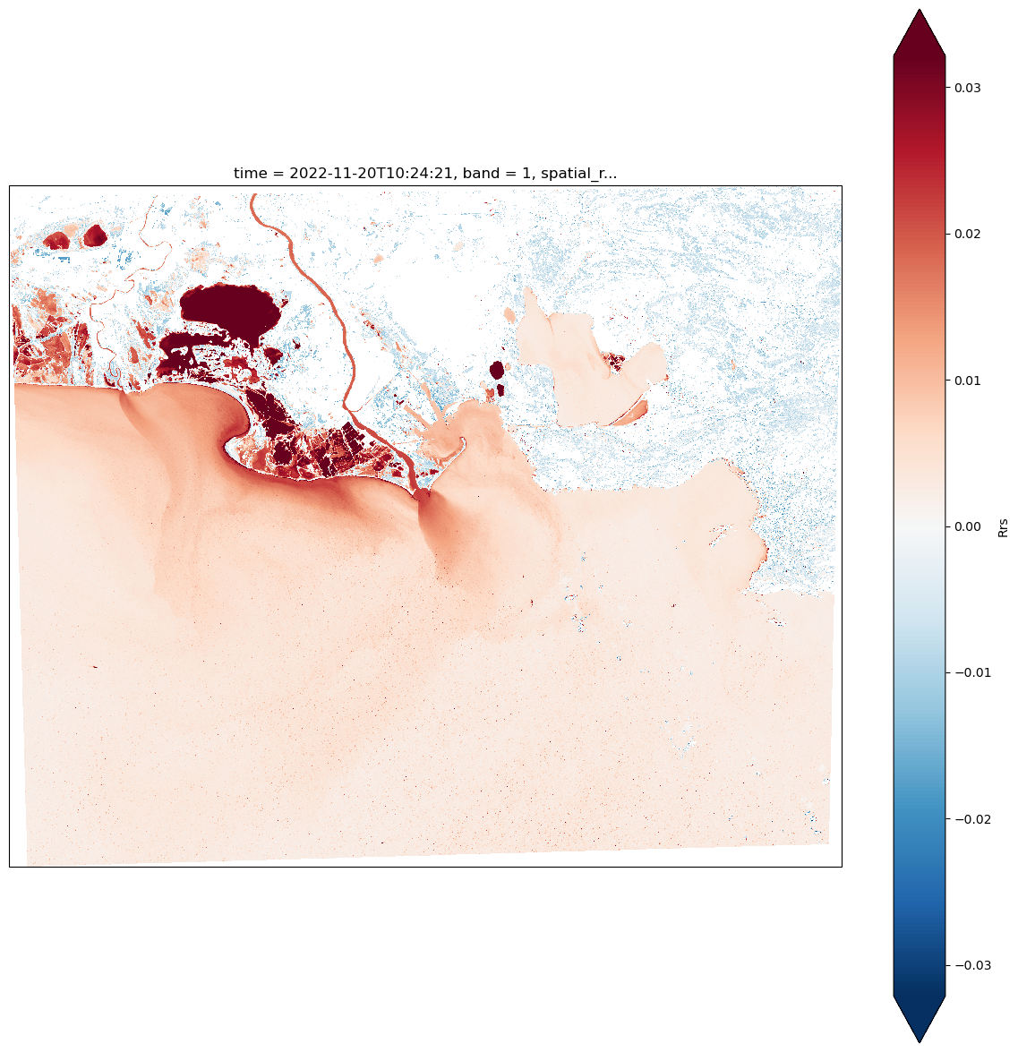
history: 2024-02-21 18:34:02 GMT by grib_to_netcdf-2.25.1: /opt/ecmw...plt.figure(figsize=(15,15))
l2_prod.Rrs.sel(wl=590).plot.imshow( robust=True,subplot_kws=dict(projection=proj))
<matplotlib.image.AxesImage at 0x7fd7ba0b3280>
plt.figure(figsize=(15,15))

l2_prod.Rrs.sel(wl=[665,560,490]).plot.imshow(rgb='wl', robust=True,subplot_kws=dict(projection=proj))
<matplotlib.image.AxesImage at 0x7fd7b9d61dc0>
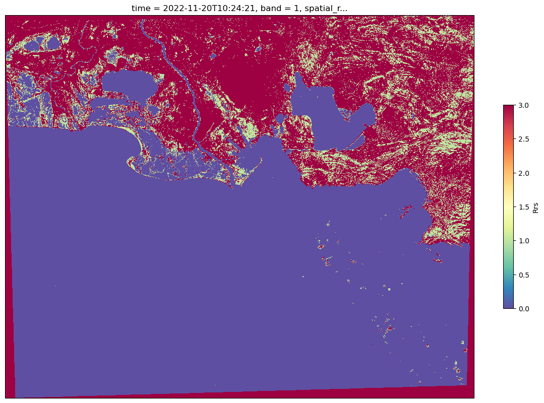
L2A to L2B#
Mask bad quality pixels#
Rrs_blue_avg=0.05
Rrs = l2_prod.Rrs
mask=xr.where((Rrs.sel(wl=490,method='nearest')<0)|(Rrs.sel(wl=565,method='nearest')<0),1,0)
mask=mask.where((Rrs.sel(wl=443,method='nearest')<2*Rrs_blue_avg),2)
mask=mask.where((Rrs.sel(wl=443,method='nearest')<3*Rrs_blue_avg),3)
#mask=mask.where((l2a.l2_prod.wv_band)<0.1,4)


plt.figure(figsize=(15,15))

mask.plot.imshow(cmap=plt.cm.Spectral_r,robust=True,subplot_kws=dict(projection=proj),cbar_kwargs={'shrink':0.35})
<matplotlib.image.AxesImage at 0x7fd7ba917c40>
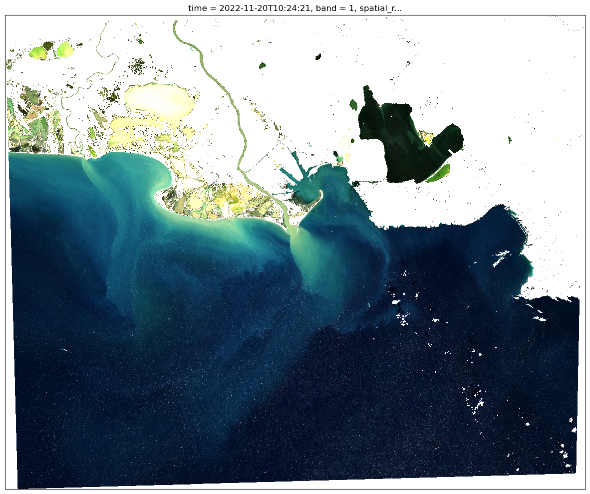
Apply mask
Rrs=Rrs.where(mask==0)
plt.figure(figsize=(15,15))
#(dem.shaded+1).plot.imshow(robust=True,subplot_kws=dict(projection=proj),cmap=plt.cm.Greys_r,cbar_kwargs={'shrink':0.4})
Rrs.sel(wl=[665,560,490]).plot.imshow(rgb='wl', robust=True,subplot_kws=dict(projection=proj))
<matplotlib.image.AxesImage at 0x7fd7ba1185b0>
Check Rrs spectra#
v=visual.view_spectral(l2_prod.Rrs,reproject=True)
v.minmax=[0,0.1]
v.visu()
geom_ = v.get_geom(v.aoi_stream,crs=prod.raster.rio.crs)

raster_clipped = xr.Dataset()
l2_prod.rio.clip(geom_.geometry.values)
for param in l2_prod.keys():
    da = l2_prod[param]
    if 'x' in da.dims and 'y' in da.dims:
        raster_clipped[param]=da.rio.clip(geom_.geometry.values)
    else:
        raster_clipped[param]=da
raster_clipped.attrs = prod.raster.attrs
---------------------------------------------------------------------------
IndexError                                Traceback (most recent call last)
Cell In[55], line 1
----> 1 geom_ = v.get_geom(v.aoi_stream,crs=prod.raster.rio.crs)
      3 raster_clipped = xr.Dataset()
      4 l2_prod.rio.clip(geom_.geometry.values)

File ~/Dropbox/Dropbox/work/git/satellite_app/grstbx/grstbx/visual.py:237, in utils.get_geom(aoi_stream, crs)
    234 @staticmethod
    235 def get_geom(aoi_stream, crs=4326):
    236     geom = aoi_stream.data
--> 237     ys, xs = geom['ys'][-1], geom['xs'][-1]
    238     polygon_geom = Polygon(zip(xs, ys))
    239     polygon = gpd.GeoDataFrame(index=[0], crs=3857, geometry=[polygon_geom])

IndexError: list index out of range
stacked = raster_clipped.Rrs.sel(wl=slice(400,1000)).stack(gridcell=["y", "x"]).dropna('gridcell',thresh=0)
---------------------------------------------------------------------------
AttributeError                            Traceback (most recent call last)
Cell In[56], line 1
----> 1 stacked = raster_clipped.Rrs.sel(wl=slice(400,1000)).stack(gridcell=["y", "x"]).dropna('gridcell',thresh=0)

File ~/anaconda3/envs/grstbx/lib/python3.9/site-packages/xarray/core/common.py:277, in AttrAccessMixin.__getattr__(self, name)
    275         with suppress(KeyError):
    276             return source[name]
--> 277 raise AttributeError(
    278     f"{type(self).__name__!r} object has no attribute {name!r}"
    279 )

AttributeError: 'Dataset' object has no attribute 'Rrs'
group_coord ='wl'
stat_coord='gridcell'
stats = xr.Dataset({'median':stacked.groupby(group_coord).median(stat_coord)})
stats['q25'] = stacked.groupby(group_coord).quantile(0.25,dim=stat_coord)
stats['q75'] = stacked.groupby(group_coord).quantile(0.75,dim=stat_coord)
stats['min'] = stacked.groupby(group_coord).min(stat_coord)
stats['max'] = stacked.groupby(group_coord).max(stat_coord)
stats['mean'] = stacked.groupby(group_coord).mean(stat_coord)
stats['std'] = stacked.groupby(group_coord).std(stat_coord)
stats['pix_num'] = stacked.count(stat_coord)
---------------------------------------------------------------------------
NameError                                 Traceback (most recent call last)
Cell In[57], line 3
      1 group_coord ='wl'
      2 stat_coord='gridcell'
----> 3 stats = xr.Dataset({'median':stacked.groupby(group_coord).median(stat_coord)})
      4 stats['q25'] = stacked.groupby(group_coord).quantile(0.25,dim=stat_coord)
      5 stats['q75'] = stacked.groupby(group_coord).quantile(0.75,dim=stat_coord)

NameError: name 'stacked' is not defined
from mpl_toolkits.axes_grid1.inset_locator import inset_axes

bands=[3,2,1]
fig, axs = plt.subplots(1,1, figsize=(10, 6))#,sharey=True


date = stats.time.dt.date.values
axins = inset_axes(axs, width="45%", height="60%",
               bbox_to_anchor=(.55, .4, 0.9, 0.9),
               bbox_transform=axs.transAxes, loc=3)


raster_clipped.Rrs.isel(wl=bands).plot.imshow(robust=True,ax=axins)
axins.set_title('')
axins.set_axis_off()
axs.axhline(y=0,color='k',lw=1)
axs.plot(stats.wl,stats['median'],marker='o',c='k')
axs.plot(stats.wl,stats['mean'],c='red',ls='--')
axs.fill_between(stats.wl, stats['q25'], stats['q75'],alpha=0.3,color='grey')
axs.set_title(date)
plt.show()
---------------------------------------------------------------------------
NameError                                 Traceback (most recent call last)
Cell In[58], line 8
      3 bands=[3,2,1]
      4 fig, axs = plt.subplots(1,1, figsize=(10, 6))#,sharey=True
----> 8 date = stats.time.dt.date.values
      9 axins = inset_axes(axs, width="45%", height="60%",
     10                bbox_to_anchor=(.55, .4, 0.9, 0.9),
     11                bbox_transform=axs.transAxes, loc=3)
     14 raster_clipped.Rrs.isel(wl=bands).plot.imshow(robust=True,ax=axins)

NameError: name 'stats' is not defined
Check water quality parameters (e.g., Chl-a concentration from diverse “algorithms”)¶#
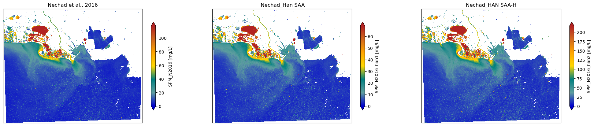
Total suspended particulate matter (SPM) from Nechad et al., 2010, 2016 formulation#
spm in mg/L#
a = [610.94*np.pi, 0.2324/np.pi]
Rrs_ = Rrs.isel(wl=3)
spm = a[0] * Rrs_ / (1 - ( Rrs_/ a[1]))
spm.name='SPM_N2016'
spm.attrs['units']='mg/L'
spm.attrs['description']='Concentration of suspended particulate matter from band 665 nm'

a = [428.277*np.pi, 0.3051/np.pi]
Rrs_ = Rrs.isel(wl=3)
spm2 = a[0] * Rrs_ / (1 - ( Rrs_/ a[1]))
spm2.name='SPM_N2016_han1'
spm2.attrs['units']='mg/L'
spm2.attrs['description']='Concentration of suspended particulate matter from band 665 nm'


a = [1444.853*np.pi, 0.3539/np.pi]
Rrs_ = Rrs.isel(wl=3)
spm3 = a[0] * Rrs_ / (1 - ( Rrs_/ a[1]))
spm3.name='SPM_N2016_han2'
spm3.attrs['units']='mg/L'
spm3.attrs['description']='Concentration of suspended particulate matter from band 665 nm'
plt.figure(figsize=(25,18))
colors = ['mediumblue','cadetblue','teal','gold','orange','chocolate','firebrick']
cmap = mpl.colors.LinearSegmentedColormap.from_list('spm',colors)
fig = plt.figure(figsize=(25, 15))
ax = plt.subplot(1, 3, 1, projection=proj)
spm.plot.imshow(cmap=cmap,ax=ax,robust=True,cbar_kwargs={'shrink':0.25},vmin=0)
ax.set_title('Nechad et al., 2016')
ax = plt.subplot(1, 3,2, projection=proj)
spm2.plot.imshow(cmap=cmap,ax=ax,robust=True,cbar_kwargs={'shrink':0.25},vmin=0)
ax.set_title(' Nechad_Han SAA')
ax = plt.subplot(1, 3,3, projection=proj)
spm3.plot.imshow(cmap=cmap,ax=ax,robust=True,cbar_kwargs={'shrink':0.25},vmin=0)
ax.set_title('Nechad_HAN SAA-H')
Text(0.5, 1.0, 'Nechad_HAN SAA-H')
<Figure size 2500x1800 with 0 Axes>
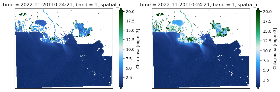
Check blue over green ratio for Chl retrieval with OC2 from NASA#
\(log_{10}(chlor\_a) = a_0 + \sum\limits_{i=1}^4 a_i \left(log_{10}\left(\frac{R_{rs}(\lambda_{blue})}{R_{rs}(\lambda_{green})}\right)\right)^i\)
# NASA OC2 fro MODIS; bands 488, 547 nm
a_modis = [0.2500,-2.4752,1.4061,-2.8233,0.5405]
# NASA OC2 for OCTS; bands 490, 565 nm
a_octs = [0.2236,-1.8296,1.9094,-2.9481,-0.1718]
# Pelevin et al, 2023, Issyk-Kul
a = [0.1977,-1.8117,1.9742,-2.5635,-0.7218]
# mona et al.
a_mona = [0.484,-2.109,2.880,-0.690,-1.040]

ratio = np.log10(Rrs.isel(wl=1)/Rrs.isel(wl=2))
chl={}
for name,a in [('nasa',a_octs),('mona',a_mona)]:
    logchl=0
    for i in range(len(a)):
        logchl+=a[i]*ratio**i
    _chl = 10**(logchl)
    _chl.name='Chla_'+name
    _chl.attrs['units']='mg.m-3'
    _chl.attrs['description']= 'Chl-a concentration from NASA OC2 with OCTS parameterization, bands 490, 565 nm',
    _chl = _chl.where((_chl >= 0) & (_chl <= 2000))
    chl[name]=_chl
import colorcet as cc
ncols=2
nrows=1
vmax=20
fig,axs = plt.subplots(nrows,ncols,figsize=(ncols*5.1,5*nrows+5),sharey=True,sharex=True,subplot_kw={'projection': proj})
fig.subplots_adjust(bottom=0.08, top=0.9, left=0.086, right=0.98,
                    hspace=0.15, wspace=0.12,)
for ii, (name,_chl) in enumerate(chl.items()):
    _chl.plot.imshow(cmap=cc.cm.CET_D13,robust=True,ax=axs[ii],cbar_kwargs={'shrink':0.35},vmax=vmax)
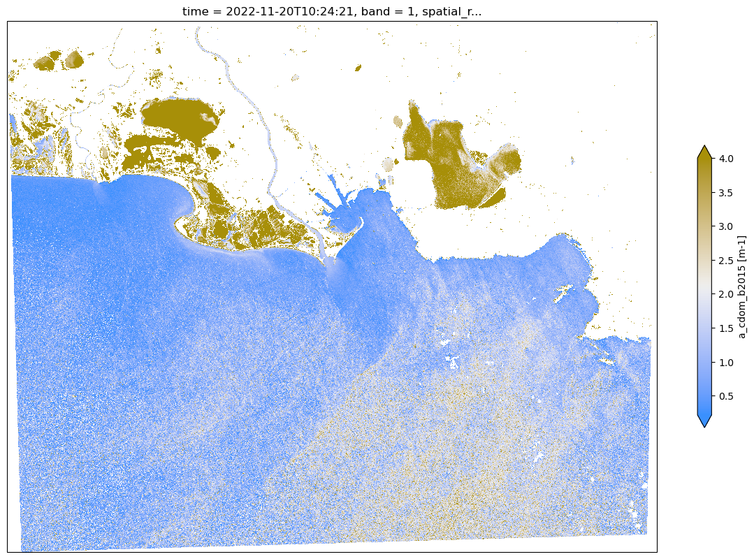
CDOM retrieval based on Brezonik et al, 2015#
a = [1.872,-0.83]
acdom = np.exp(a[0] + a[1] * np.log(Rrs.isel(wl=1)/Rrs.isel(wl=5)))
acdom.name='a_cdom_b2015'
acdom.attrs['units']='m-1'
acdom.attrs['description']='CDOM absorption at 440 nm-1'
acdom= acdom.where((acdom >= 0) & (acdom <= 60))
plt.figure(figsize=(15,15))

acdom.plot.imshow(cmap=cc.cm.CET_CBD1,robust=True,subplot_kws=dict(projection=proj),cbar_kwargs={'shrink':0.35},vmax=4)
<matplotlib.image.AxesImage at 0x7fd788389190>
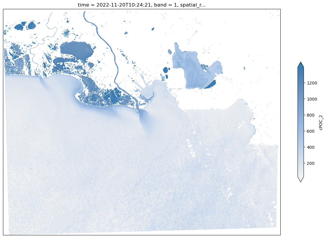
def cPOC_2(Rrs,p=[2.873,0.945,0.025]):
    ratio1=Rrs.sel(wl=665,method='nearest') / Rrs.sel(wl=490,method='nearest')
    ratio2=Rrs.sel(wl=665,method='nearest') / Rrs.sel(wl=565,method='nearest')
    ratio = np.log10(xr.concat([ratio1.assign_coords({'num':1}),ratio1.assign_coords({'num':2})],dim='num').max('num'))

    Xpoc = p[0]+p[1]*ratio+p[2]*ratio**2
    return 10**Xpoc

poc = cPOC_2(Rrs)
poc.name = 'cPOC_2'
plt.figure(figsize=(15,15))

poc.plot.imshow(cmap=cc.cm.blues,robust=True,subplot_kws=dict(projection=proj),cbar_kwargs={'shrink':0.35})
<matplotlib.image.AxesImage at 0x7fd788327220>
Check Optical Water Types (OWT)#
owt_file = ‘/DATA/projet/vrac/owt/Spyrakos_et_al_2018_OWT_inland_mean_standardised.csv’ owt =pd.read_csv(owt_file,index_col=0).stack().to_xarray() owt = owt.rename({‘level_1’:‘wl’}) owt[‘wl’]=owt.wl.astype(float)
import matplotlib.patches as mpatches
owt_info={ 1:dict(color=‘olivedrab’,label=‘OWT1: Hypereutrophic waters’), 2:dict(color=‘black’,label=‘OWT2: Common case waters’), 3:dict(color=‘cadetblue’,label=‘OWT3: Clear waters’), 4:dict(color=‘tan’,label=‘OWT4: Turbid waters with organic content’), 5:dict(color=‘chocolate’,label=‘OWT5: Sediment-laden waters’), 6:dict(color=‘teal’,label=‘OWT6: Balanced optical effects at shorter wavelengths’), 7:dict(color=‘blueviolet’,label=‘OWT7: Highly productive cyanobacteria-dominated waters’), 8:dict(color=‘plum’,label=‘OWT8: Productive with cyanobacteria waters’), 9:dict(color=‘red’,label=‘OWT9: OWT2 with higher \(R_{rs}\) at shorter wavelengths’),#‘slategrey’ 10:dict(color=‘orange’,label=‘OWT10: CDOM-rich waters’), 11:dict(color=‘gold’,label=‘OWT11: CDOM-rich with cyanobacteria waters’), 12:dict(color=‘firebrick’,label=‘OWT12: Turbid waters with cyanobacteria’), 13:dict(color=‘mediumblue’,label=‘OWT13: Very clear blue waters’), } colors = [‘olivedrab’,‘black’,‘cadetblue’,‘tan’,‘chocolate’,‘teal’,‘blueviolet’,‘plum’,‘red’,‘orange’,‘gold’,‘firebrick’,‘mediumblue’] cmap_owt = mpl.colors.ListedColormap(colors)
patch = [] for key,info in owt_info.items(): patch.append(mpatches.Patch(color=info[‘color’], label=info[‘label’]))
fig, ax = plt.subplots(nrows=1,ncols=1, sharex=True,figsize=(9, 6)) ax.minorticks_on() for iowt,group in owt.groupby(‘owt’):
group.plot(color=owt_info[iowt]['color'],lw=3)
ax.set_title(‘’ )
ax.set_ylabel(‘\(Standardized\ R_{rs}\ (nm^{-1})\)’,fontsize=20)
ax.set_xlabel(‘\(Wavelength\ (nm)\)’,fontsize=20)
plt.legend(handles=patch,fontsize=13,bbox_to_anchor=(1, .5, 0.5, 0.5))
def SAM(R1,R2): denum=(R1*R2).sum(‘wl’) denom = (R1**2).sum(‘wl’)0.5 * (R22).sum(‘wl’)**0.5 return np.arccos(denum/denom)
def SCS(R1,R2): R1_avg = R1.mean(‘wl’) R2_avg = R2.mean(‘wl’) R1_std = R1.std(‘wl’) R2_std = R2.std(‘wl’) Nwl = len(R1.wl) return 1/(Nwl) * ((R1-R1_avg) * (R2-R2_avg)).sum(‘wl’) / (R1_std*R2_std)
Rrs_sat = Rrs.sel(wl=slice(350,800))#.dropna(‘wl’)
Rrs_owt = owt.interp(wl=Rrs_sat.wl)
owt_sam = SAM(Rrs_sat,Rrs_owt) owt_scs =SCS(Rrs_sat,Rrs_owt)
owt_delta = owt_scs + (1-2*owt_sam/np.pi)/2
fig = plt.figure(figsize=(25, 15)) ax = plt.subplot(1, 2, 1, projection=proj)
cmap = plt.get_cmap(‘tab20c’,13) (owt_delta.fillna(-1).argmax(‘owt’)+1).where(Rrs_sat.isel(wl=1)>0).plot.imshow(vmin=0.5,vmax=13.5,cmap=cmap_owt,cbar_kwargs={ ‘ticks’:range(1,14),‘shrink’: 0.4},ax=ax) ax = plt.subplot(1, 2, 2, projection=proj) cmap = plt.get_cmap(‘RdBu’)#,13) (owt_delta.max(‘owt’)).where(Rrs_sat.isel(wl=1)>0).plot.imshow(robust=True,cmap=cmap,ax=ax, cbar_kwargs={ ‘shrink’: 0.4})
#l2b.to_netcdf('/DATA/vrac/test_l2b.nc')